Introduction
This blog is a new function, treatment_model that have been added to the Dyn4cast package. The function provides means for enhanced estimation of propensity score and treatments effects from randomized controlled designed experiments.
Observational study involves the evaluation of outcomes of participants not randomly assigned treatments or exposures. To be able to assess the effects of the outcome, the participants are matched using propensity scores (PSM). This then enables the determination of the effects of the treatments on those treated against those who were not treated. Most of the earlier functions available for this analysis only enables the determination of the average treatments effects on the treated (ATT) while the other treatment effects are optional. This is where this functions is unique because five different average treatment effects are estimated simultaneously, in spite of the one line code arguments. The five treatment effects are:
Average treatment effect for the entire (ATE) population
Average treatment effect for the treated (ATT) population
Average treatment effect for the controlled (ATC) population
Average treatment effect for the evenly matched (ATM) population
Average treatment effect for the overlap (ATO) population.
There excellent materials dealing with each of the treatment effects, please see
The basic usage of the codes are:
treatment_model(Treatment, x_data)
Arguments
Treatment Vector of binary data (0, 1) LHS for the treatment effects estimation
x_data Data frame of explanatory variables for the RHS of the estimation
Let us go!
Load library
library(Dyn4cast)Estimation of treatment effects model
Treatment <- treatments$treatment
data <- treatments[, c(2:3)]
treat <- treatment_model(Treatment, data)
Estimated treatment effects model
summary(treat) Length Class Mode
P_score 500 -none- numeric
Effect 5 data.frame list
Fitted_estimate 500 -none- numeric
Residuals 500 -none- numeric
Model 30 glm list
Experiment plot 11 gg list
ATE plot 11 gg list
ATT plot 11 gg list
ATC plot 11 gg list
ATM plot 11 gg list
ATO plot 11 gg list
weights 5 data.frame list Estimated various treatment effects
treat$Effect ATE ATT ATC ATM ATO
1 2.465581 4.481578 -0.2272903 1.968055 2.056329Estimated propensity scores from the model
head(treat$P_score) 1 2 3 4 5 6
0.98347730 0.97153060 0.63093981 0.69944426 0.07971976 0.90935715 ##Ffitted values from the model
head(treat$Fitted_estimate) 1 2 3 4 5 6
0.98347730 0.97153060 0.63093981 0.69944426 0.07971976 0.90935715 Residuals of the estimated model
tail(treat$Residuals) 495 496 497 498 499 500
-2.250645 -1.757826 1.402062 1.010765 -1.151789 1.898509 Plots of the propensity scores from the model
Quite a number of plots are in the works e.g.
Treatment effects (ATE)
treat$`ATE plot`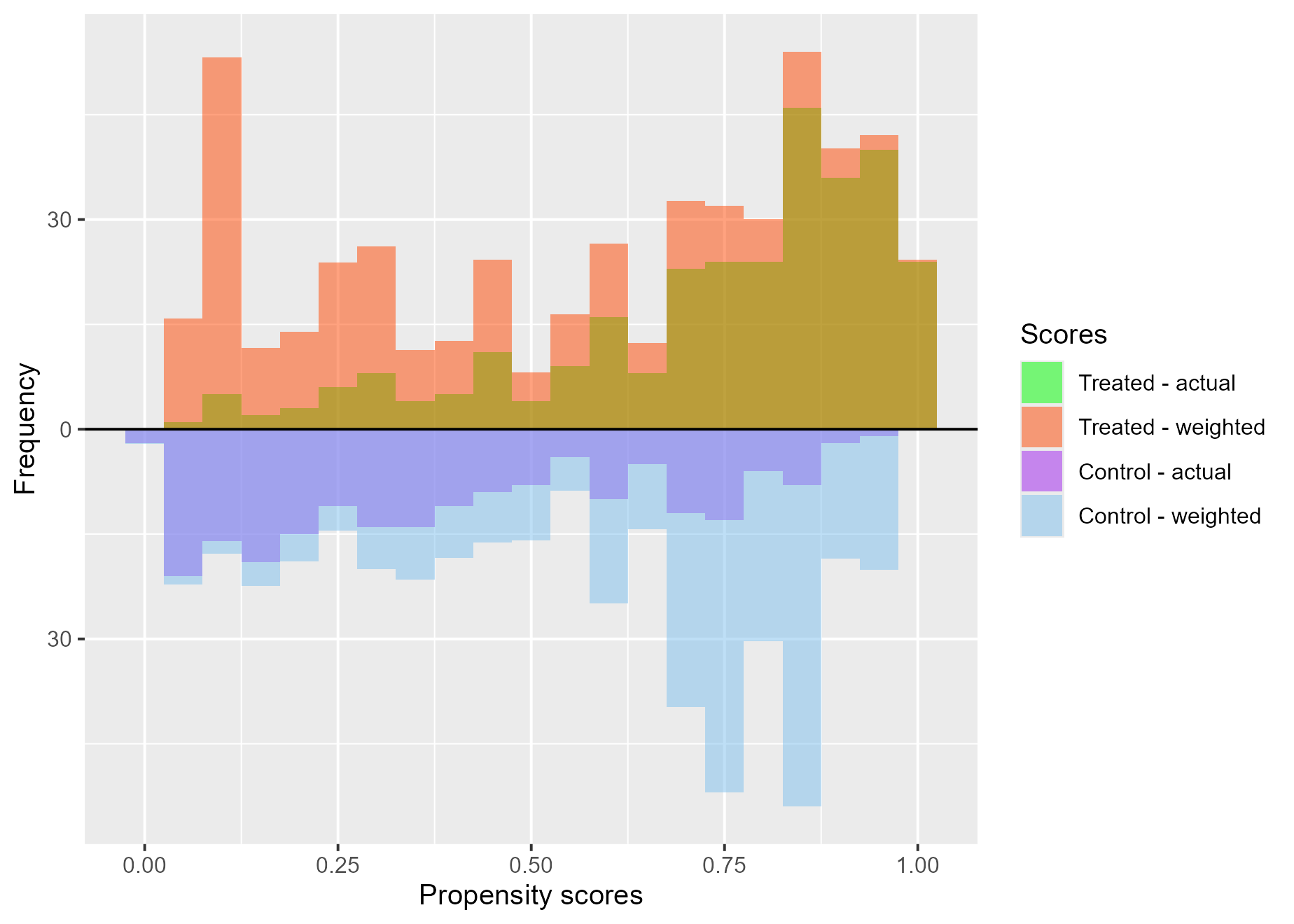
Treatment effects on the treated (ATT)
treat$`ATT plot`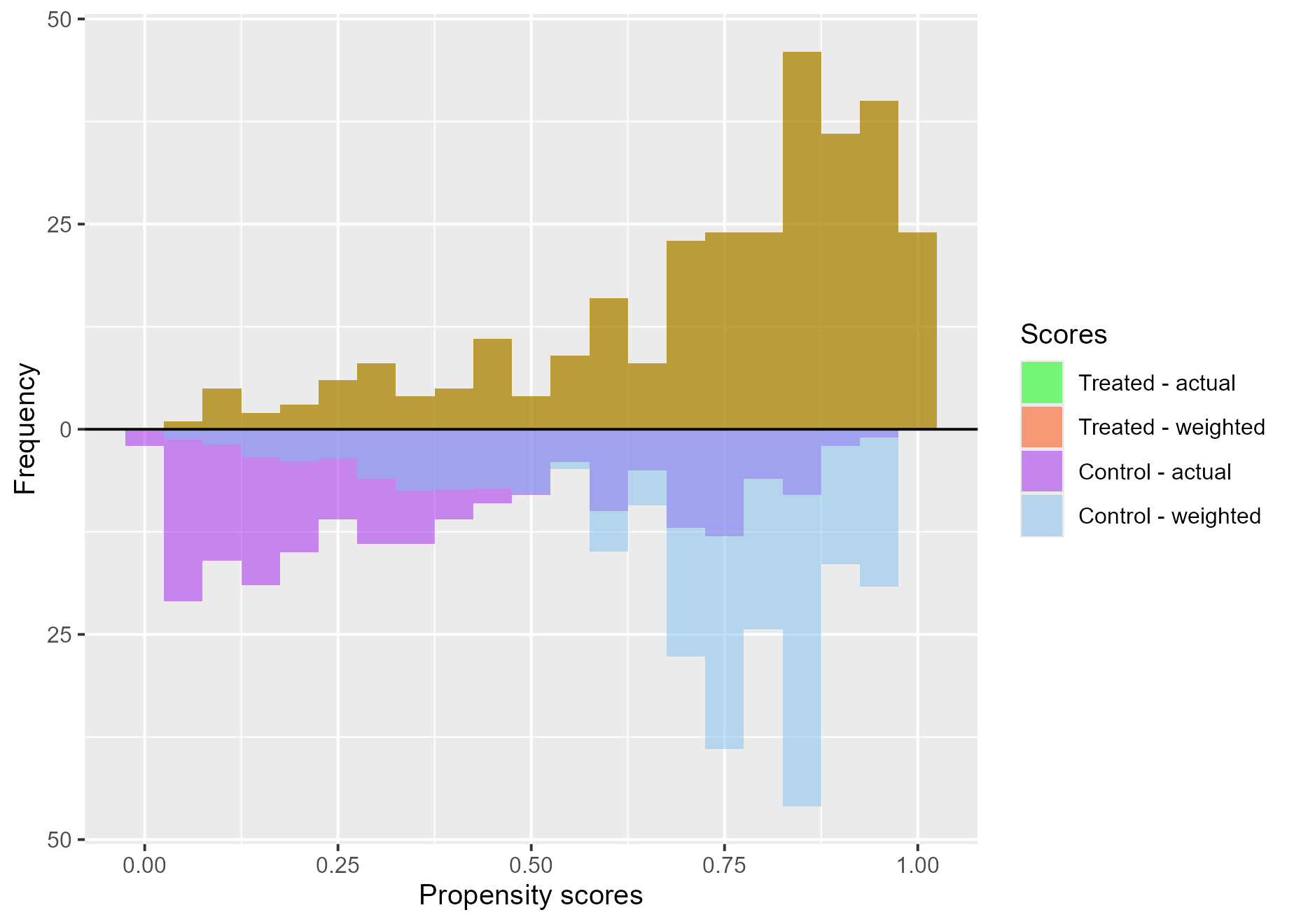
Treatment effects on the evenly matched (ATM)
treat$`ATM plot`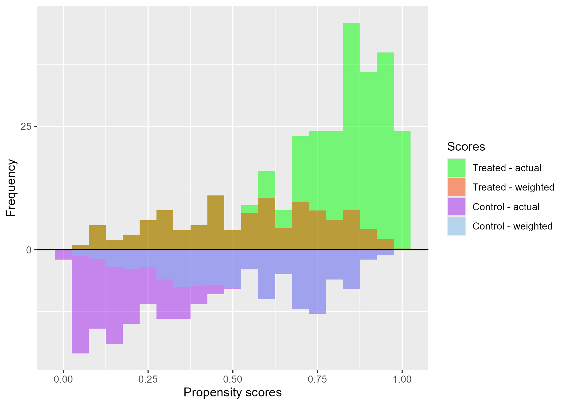
Welcome to the world of easy Data Science and easy Machine Learning!